One of Charlie's interests is remote sensing and environmental monitoring; there are several interesting applications:
- gathering ecological data, such as the meteorological (temperature, humidity), the biological (animal noises), and the anthropological (light pollution from encroaching development). You can read some more about this here at Charlie's blog or at this archived ArkFab post.
- Monitoring and automation of food production facilities, such as mycoponics and aquaponics, greenhouses, and apiaries.
- Smart homes
This project aims to build a basic platform for monitoring the local environment, and ultimately build greenhouse and beehive monitors.
Adafruit provides combined temperature and humidity sensors, the DHT series. Although we have one of the nicer DHT22 sensors, let's start off using the less expensive (though less precise and more limited) DHT11.
One quantity that might be interesting to measure is the difference in temperature and humidity between a controlled environment like a greenhouse, and a reference environment, like the outdoors. To measure this, it'll be important to compare the two sensors under identical conditions, to get an idea of the bias and noise between them.
For monitoring light levels, we'll start off using CdS-based photoresistors.
Eventually, it'll be good to look into WiFi and SD card shields for data logging and solar-powered battery packs for long-term, remote operation.
For beehive monitoring, we'll also want to get a scale with digital strain sensors.
Here's a github repository to track the project's code and data:
https://github.com/Recybery/basic_environmental_monitoring
Here's about a day's worth of data from a single DHT11 sensor, some distance from a heat duct but in its direct path:
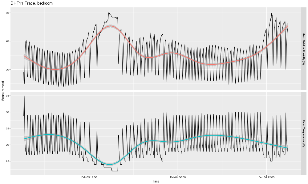
Clock time is the horizontal axis; the upper pane tracks relative humidity in percent, and the lower pane tracks temperature in degrees celcius. Much of the variation is due to an oscillation of about 30 minutes, with the sensor cooling and growing more humid until a spike of hot, dry air appears. This is the furnace cycling on and off. During the afternoon, the oscillations stop, but the temperature continues to drop. This is because the thermostat is in the living room, which gets direct sun; the sensor was in a rear room which is shaded. The living room stayed warm enough to keep from tripping the thermostat while the rear room, separated with a closed door, cooled.
There are lower-frequency changes too; the step-change in both temperature and humidity on midnight of the second day corresponds to a rainstorm arriving, for example.
Sometimes we'll want to record two different sets of measurements. For example, taking temperature measurements inside a greenhouse and comparing them to an external reference temperature will establish how much warmer the greenhouse is than the outside. Even when one measurement is being taken, it's good to have an idea of the inter-instrument variation. Here's a time series of temperature and humidity, taken simulatenously with two DHT11 sensors sitting side by side:
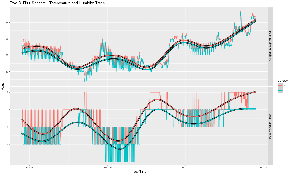
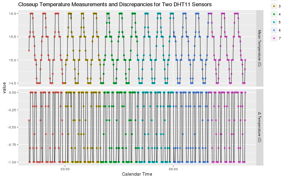
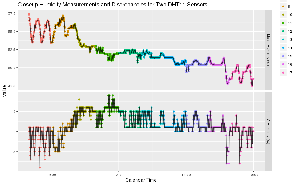
This shows a similar pattern as before, with warm, dry days and high-frequency signal from the furnace on the cool nights. It's also clear that there is an offset between the two sensors, both for the temperature and the humidity measurements. It looks as though the offset is smaller in the humidity signal, compared to the variation. We can explore this relative bias between the two sensors by subtracting one reading from the other, to generate new time series consisting of the difference between sensors. Here the difference in temperature and humidity readings are plotted over time, with hour of the day represented using color:
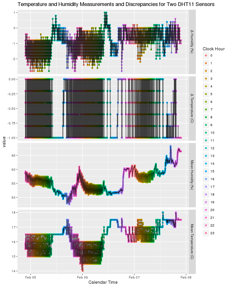
Looking at the difference between sensors (top two facets), there is a clear relationship between the inter-sensor bias and the furnace behavior. During the day (approx. 10AM to 6 PM), regular furnace cycling stops and the difference in temperature measurement between the sensors settles on a consistent -1 C. When the furnace begins cycling, the temperature difference begins fluctuating as well, between the reexisting -1 and 0 C. However, the fluctuation in temperature discrepancy has a greater frequency than the oscillation of temperature itself, suggesting it's not just the furnace cycle driving it.
Humidity has a more complicated behavior: with the furnace cycling, the humidity difference varies between -1 and -2 percent between the two sensors. When the furnace stops cycling in the midday, the discrepancy jumps to almost 0 between them, then slowly relaxes back to the previous offset by the time the furnace cycle resumes.
cereal=$1
#e.g., /dev/ttyACM1
phial_out=$2
ttylog -b 9600 -d "$cereal" -f |  ts '%Y-%m-%d	%H:%M:%S' | tee "$phial_out"
Here's some of the details of the code: the DHT11 and library report the measurements directly, which the Arduino reports to the serial port. Computerside, the above bash script monitors the serial port with ttylog. In the wild, timestamping would happen Arduino-side; here it was accomplished by piping the serial port output through the moreutils ts command before storing.
Another design aspect is the sampling structure. Here's the Arduino code responsible:
int burst = 0;
int replicate_number = 5; // how many replicates per burst
int rep_delay = 2; // how many delayMS units to wait between replicates
int burst_delay = 60; // how many seconds between measurements


void loop() {
for (int counter = 0; counter < replicate_number; counter++){
  // Delay between replicates
  delay(delayMS*rep_delay);
  // Get temperature event and print its value.
  sensors_event_t event;
  dht.temperature().getEvent(&event);
    Serial.print(burst);
    Serial.print("  ");

    Serial.print(counter);
    Serial.print("  ");

    Serial.print(event.temperature);
    Serial.print("  ");

    dht.humidity().getEvent(&event);
    Serial.print(event.relative_humidity);

    Serial.println(" ");
    }
  burst += 1;
  delay(burst_delay);
 }
The environment is sampled with an interval ofburst_delay seconds; each sampling consists of replicate_number measurements, with a delay of rep_delay minimum delay units. The loop() function keeps a running count of the burst number, and a rolling count of the counter number, both of which are reported alongside the sensor readings. After some minor munging, the data looks something like this:
date    time    burst   replicate temp    hum
2018-02-03      03:09:43        0       0       28.00   18.00
2018-02-03      03:09:45        0       1       29.00   18.00
2018-02-03      03:09:47        0       2       29.00   18.00
2018-02-03      03:09:50        0       3       29.00   18.00
2018-02-03      03:09:52        0       4       29.00   18.00
2018-02-03      03:10:24        1       0       29.00   18.00
2018-02-03      03:10:26        1       1       30.00   15.00
2018-02-03      03:10:29        1       2       30.00   15.00
2018-02-03      03:10:31        1       3       30.00   15.00
2018-02-03      03:10:33        1       4       30.00   15.00
2018-02-03      03:11:06        2       0       30.00   14.00
2018-02-03      03:11:08        2       1       31.00   13.00
2018-02-03      03:11:10        2       2       31.00   13.00
2018-02-03      03:11:12        2       3       31.00   13.00
2018-02-03      03:11:15        2       4       31.00   12.00
...
Once in this form, the data is ready to be processed through the tidyr framework. For example, the date and and time can be merged into a temporal object using the lubridate:
single_sensor_test <- data.frame(single_sensor_test)
single_sensor_test$date<- ymd(single_sensor_test$date)
single_sensor_test$time<- hms(single_sensor_test$time)
single_sensor_test$dateTime <- single_sensor_test$date + single_sensor_test$time
single_sensor_test$dateTime<- as.POSIXct(single_sensor_test$dateTime)
The five replicates in each burst can be easily summarized using dplyr's group_by and summarize:
single_sensor_test.summarized <- single_sensor_test %>% group_by(burst) %>% summarize(meanTime = mean(dateTime), meanTempC = mean(tempC), meanRelHum=mean(relHum))
There are a few reasons to take measurements this way, rather than constantly sampling or taking single samples. The first method could be inefficient at high sampling frequency, requiring large storage space for redundant data. Single samples, on the other hand, might result in a noisier signal, since instrumental variability wouldn't get averaged out at all. Another potential advantage is the counterintuitive fact that repeated sampling can give an estimate with a higher precision than that of the measurements themselves.
As long as we're adding sensors, we might want to monitor light levels as well. A simple approach is to use a standard CdS photoresistor with a constant voltage and measure the remainder on an analog-in pin. Here, the trace is plotted on a background shaded to indicate the ambient temperature. When light strikes the CdS cell, its resistance drops, and it registers a higher value on the analog pin. In the dark, the resistance is high, and the reading at the pin is low. The diurnal cycle in both temperature and luminosity is thus visible:
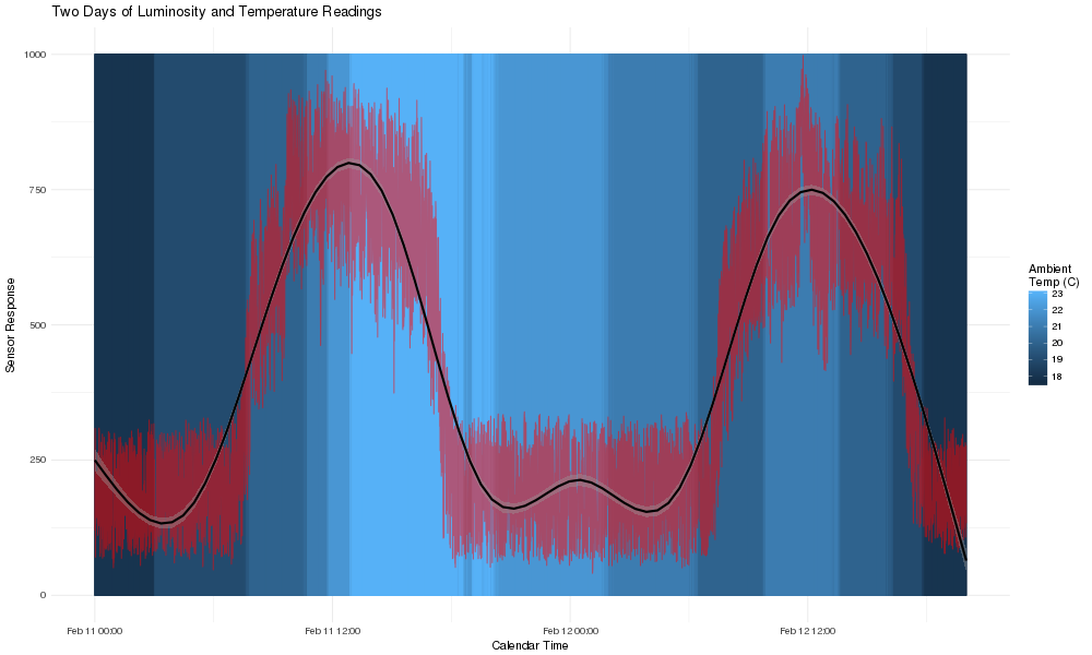
This seems to work well at distinguishing between moderate levels of lighting, but it might not be good for distinguishing low levels (like the difference between a full and a new moon) or small differences (like changes in cloud cover over the course of a day). A more advanced option might be the TSL2591 sensor.
A lot of work has been going on behind the scenes on this project, but I've been waiting to get a decent dataset for measuring scale drift before posting here. Along the way, this has meant:
- moving time-stamping off of the computer-side serial connection and onto the board itself using an RTC module
- using on-board USB logging, eventually turning to a logging shield
- adding a weight sensor using a repurposed bathroom scale
- experimenting with mobile power supplies
The logger was run for about a week and a half at a sampling frequency of about 5 minutes, with six replicates per sample burst. A known weight (1 gallon of water = 8.34 lb = 3.785 kg) was placed on the scale. The purpose was primarily to get information on how the scale's measurement of a constant weight would fluctuate. Instrumental drift is apparently a concern when the load cells of the scale are used continuously for long periods. Once the replicates are averaged into burst values, the weight measurements look like this:
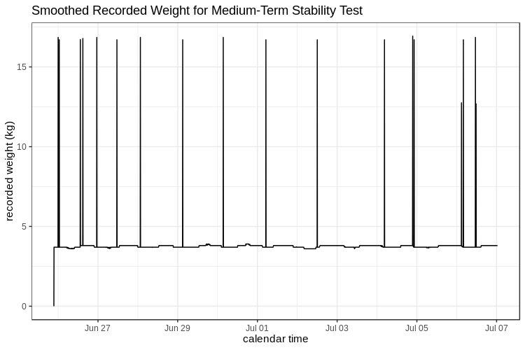
Scaled to their range, the weight measurents are relatively steady: there is the step-up at the start of the time series, when the gallon jug of water was placed on the tared scale. There are also a very small number of transient spikes into values higher by a factor of 3. It's not obvious where these are coming from. They appear to be distributed evenly throughout the day:
> inner_join(timeLapse, timeLapse.summarized %>% filter(meanWt >5) %>% select(burst), by = c("burst"="burst")) %>% select(date) %>% summary()
      date
 Min.   :2019-06-26
 1st Qu.:2019-06-26
 Median :2019-06-30
 Mean   :2019-06-30
 3rd Qu.:2019-07-04
 Max.   :2019-07-06

>inner_join(timeLapse, timeLapse.summarized %>% filter(meanWt >5) %>% select(burst), by = c("burst"="burst")) %>% select(time) %>% summary()
      time
 Min.   :1M 0S
 1st Qu.:3H 0M 55.75S
 Median :8H 11M 26.5S
 Mean   :9H 16M 30.32S
 3rd Qu.:13H 22M 17.25S
 Max.   :23H 17M 55S
Looking at the raw data, it appears that these spikes are caused by individual bad replicates within a measurement burst. These can be excluded, and the average value calculated on the "good" replicates. This means that we can still rescue a reasonable data point from a burst with a bad replicate, although the measurement will have a smaller sample size. Most mysteriously, the bad replicates are not evenly distributed among the measurements taken, but only occur in the third and fifth measurements in a burst!
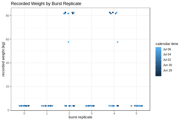
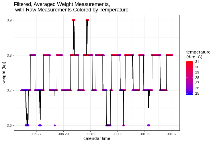
Although these spikes are extreme, there are very few of them. In fact, of 2800 averaged measurements, only 18 (~0.6%) were such obvious outliers. When filtered to remove them, and the initially empty scale, we get a periodic oscillation of measured weight, mostly between 3.7 and 3.8 kg, with excusrions as far as 3.6 or 3.9. The raw data have also been included, which fall into discrete 0.1 kg increments, and have been colored with their measured temperature to indicate a likely culprit: many electronic devices change their behavior slightly with temperature. As we continue working on this project, a goal will be finding a model to correct the measured weight based on measured temperature. All in all though, this is reassuring: there doesn't seem to be a lot of unmanageable instrumental drift on the scale of days-to-weeks!
